Translation of maspy's Slope Trick
Note: this is a translation of maspy’s article Slope Trick. The translation is done with the aid of deepl and is known to be incomplet and incorrekt.
Original article (in Japanese) by maspy.
Piecewise linear convex functions
Definition
The slope trick is a technique to manage a continuous function \(f\colon \R \to \R\) which satisfies the following condition.
The graph of \(f\) is a polyline joining line segments with slopes \(l, l + 1, \dots, r - 1, r\) in this order from left to right.
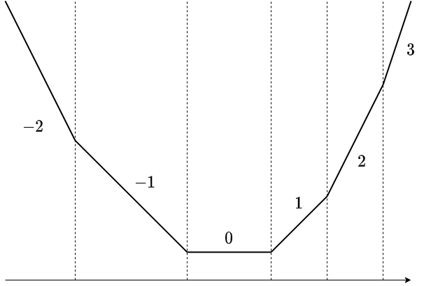
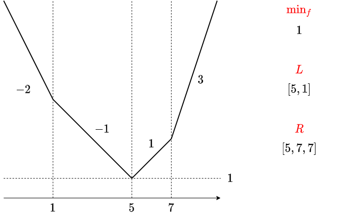
It is like this. This is a line segment with slopes of \(-2, -1,0, 1, 2, 3\). It is called a line segment, although both ends are half line.
For convenience, we will also consider a line segment of length \(0\).
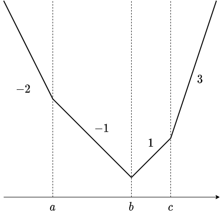
In the above figure,
- in \((-\infty, a]\) the slope is \(-2\)
- in \([a, b]\) the slope is \(-1\)
- in \([b, b]\) the slope is \(0\)
- in \([b, c]\) the slope is 1
- in \([c, c]\) the slope is \(2\)
- in \([c, \infty)\) the slope is \(3\)
Hereafter, we will refer to such functions as piecewise linear convex functions. Strictly speaking, segmented linear convexity alone is insufficient, since we require the slope to be integer, but we don’t think there will be any confusion in this article. Please understand.
Examples
The following are some examples of piecewise linear convex function.
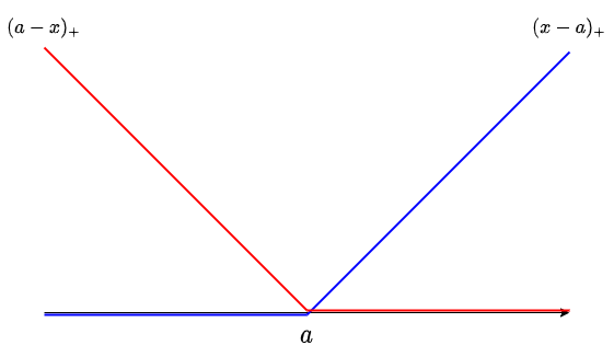
- \(f(x) = |x - a|\)
- \(f(x) = \max(0, x - a)\). Hereinafter referred to as \((x - a)_+\).
- \(f(x) = \max(0, a - x)\). Hereinafter referred to as \((a - x)_{+}\).
We will visualize the last two functions, which are particularly important. These are the left and right halves of \(|x - a|\), for which we have \(|x - a| = (x - a)_{+} + (a - x)_{+}\).
We also see that the sum of some piecewise linear convex functions is a piecewise linear convex function. Thus, for example, a function such as \(f(x)= \sum_i|x-a_i|\) is a piecewise linear convex function.
How to hold the data
The slope trick is to manage piecewise linear convex functions by replacing them with a multiset of slope change points, so that certain function operations can be performed concisely.
There seem to be a number of possible patterns in the details of the data. For example, in https://codeforces.com/blog/entry/77298 you can see some attempts to describe functions in terms of change points and how they look in \(x \to \infty\). In this article, I will introduce what I consider to be an easy way to handle the data.
Data representation
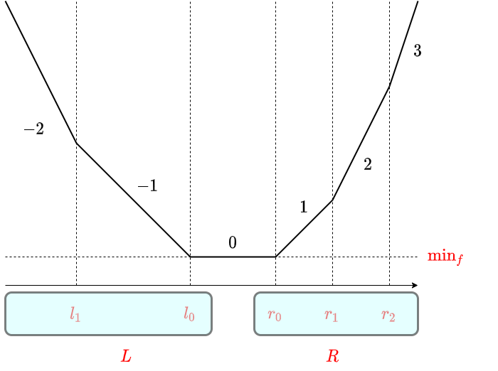
For a piecewise linear convex function, we have the following three pieces of information
- \(\min_f\): the minimum value of \(f\)
- \(L\): a multiset of all points of change in slope, for the part with slope \(\le 0\).
- \(R\): a multiset of all points of change in slope, for the part with slope \(\ge 0\).
In the following, we always write \(l_0\) to indicate the maximum value of \(L\), and \(r_0\) to indicate the minimum value of \(R\). Also, if \(L\) or \(R\) is empty, set \(l_0=-\infty\) or \(r_0=\infty\), respectively. The way to represent a “multiset” is to use a priority queue so that \(l_0\) and \(r_0\) are always available.
This is an example of where the slope changes by more than \(1\) at a point.
Restoration
With the above way of holding data, \(f(x)\) can be expressed as follows: \[ f(x) = \text{min}_{f} + \sum_{l\in L} (l-x)_{+} + \sum_{r \in R} (x-r)_{+} \] In fact, on the left and right sides
the slopes are equal everywhere
the values are equal at \(x\in [l_0,r_0]\)
Both are easy to verify.
Possible operations
Let \(N=|L|+|R|\). In this case, the following operations and computational complexity can be achieved.
Obtain minimum value: \(O(1)\) time
\(\min_{x\in\R} f(x)\) and other such questions about \(x\) can be answered in \(O(1)\) time. (这句翻译不通,原文“\(\min_{x∈\R}f(x)\) および、それを実現するような \(x\) を答えることが、\(O(1)\) 時間で行えます。”)Since we were talking about managing \(\min_f\) in the first place, we will just return the minimum value. The range of \(x\) that takes the minimum value is the interval \([l_0,r_0]\) with slope \(0\), which can be obtained in \(O(1)\) time since it only reads the top of the priority queue.
Add a constant \(a\): \(O(1)\) time
Just add \(a\) to \(\min_f\). It’s a no-brainer.
Add \((x - a)_{+}\): \(O(\log N)\) time
If we add this, \(a\) is added to the set of points where the slope changes. Also, since the minimum value of the slope does not change and the maximum value changes by \(+1\), the size of \(L\) remains the same, while the size of \(R\) increases by \(1\). (Denote the size of \(L\) and \(R\) before the operation as \(N_L\) and \(N_R\) respectively.) Therefore, we can cut the multiset \(L∪R∪{a}\) into two parts, starting from the smallest one, (the \(N_L\) smallest points forms the new \(L\) the remaining \(N_R + 1\) points forms the new \(R\)) and denote them as \(L\) and \(R\) again. For example, it can be updated by the following procedure.
- Push \(a\) to \(L\).
- Pop a value from \(L\) and push it to \(R\).
If \(a \ge l_0\), the first push is useless, so you can divide the case by the relationship between \(a\) and \(l_0\). Alternatively, if you have a method that does push/pop together as a priority queue operation, there is almost no waste even when \(a \ge l_0\). For example, the standard python library heapq can be implemented by calling heappushpop / heappush one at a time. (原文:例えば python の標準ライブラリ heapq であれば、heappushpop / heappush を一度ずつ呼ぶ形で実装できます。)
Now that we know how to update \(L\) and \(R\), let’s consider updating \(\min_f\). Although it may seem troublesome to separate cases based on the position of \(a\), it is actually quite simple. We will focus on (the value of) \(f\) at the maximum value of \(L\) before the update, \(l_0\).
Actually, even after the update, \(l_0\) is the point that gives the minimum value. In fact, with the insertion of \(a\), the slope before and after \(l_0\) changes by either \(+0\) or \(+1\). Since \(l_0\) was the boundary point with slope \(-1,0\) before the update, it will be the boundary point with slope \(-1,0\) or \(0,1\) after the update. Therefore, the change in \(\min_f\) is equal to the change in \(f(l_0)\), and
- \(\min_f \gets \min_f+(l_0−a)_+\)
and the update of the minimum value is complete.
Add \((a - x)_{+}\): \(O(\log N)\) time
It’s the same.
- \(\min_f \gets \min_f+(a-r_0)_{+}\)
- push \(a\) to \(R\)
- pop one value from \(R\) and push it to \(L\)
Add \(|x - a|\): \(O(\log N)\) time
\(|x-a|=(x-a)_+ + (a-x)_+\), so we can do both of the above operations in any order we like.
Cumulative min: \(O(1)\) time
In other words, it is an operation to replace \(f\) with \(g\) as \(g(x):=\min_{y≤x} f(y)\).
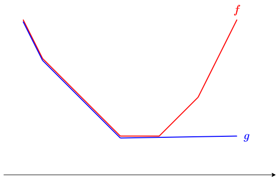
We can replace \(R\) with the empty set.
Cumulative min from right
\(g(x):=\min_{y≥x} f(y)\), this operation replaces \(f\) with \(g\).
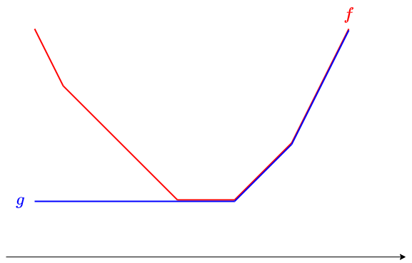
We can replace \(L\) with the empty set.
Extensions
If we add additional information to the data structure, we can perform more operations. Specifically, in addition to \(\min_f\), \(L\), and \(R\), we will add \(\mathrm{add}_L\) to the left side, and \(\mathrm{add}_R\) to the right side.
When inserting or extracting, take care of the difference between the actual values and the values you are putting in \(L\) and \(R\). By doing so, we can perform addition to the entire left and right sets in \(O(1)\) time.
Let’s see how the operation can be done.
Horizontal shift: \(O(1)\) time
Given a piecewise linear convex function \(f(x)\), we consider finding a function \(g\) such that \(g(x)=f(x-a)\).
![]()
We can add \(a\) to the sets \(L\) and \(R\) all at once.
Sliding window minimum: \(O(1)\) time
This operation takes the sliding window minimum.
For \(a≤b\), compute \(g\) determined by \(g(x)=\min_{y \in [x-b,x-a]}f(y)\).
This actually corresponds to translating the left and right sets, respectively.
![]()
I think it makes sense from a graphical point of view to take min for all the translations between \(a\) and \(b\). Just to be sure, let’s understand it in terms of equations.
- If \(x≤l_0+a\), then \(f\) is monotonically decreasing in \([x-b,x-a]\) from \(x-a \le l_0\). Therefore \(g(x)=\min_{y \in [x-b,x-a]} f(y) = f(x-a)\).
- If \(x≥r_0+b\), then \(x-b≥r_0\) and \(f\) is monotonically increasing in \([x-b,x-a]\). Thus \(g(x) = \min_{y \in [x-b,x-a]} f(y) = f(x-b)\).
- If \(l_0 + a \le x \le r_0 + b\), then \([x-b,x-a] \cap [l_0,r_0] \ne \O\), so \(g(x) = \min_f\).
In addition, horizontal shift can be regarded as the \(a=b\) case of this.
Also, the operation of taking cumulative min can be regarded as the case where \(b = \infty\). However, adding or subtracting \(\infty\) many times will make the operation suspicious, and replacing \(\infty\) with a sufficiently large constant will cause concerns about overflow and calculation errors, so I think it is better to simply implement \(R\) to be empty.